Gantt chart in Excel without add-ins: conditional formatting, step by step

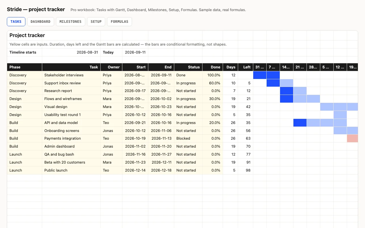
A Gantt bar is a row of cells whose weeks overlap a task's dates. That's one AND() in a conditional-format rule. Two more rules give you the done share and blocked tasks; a fourth marks today.

Contents

A task list with Gantt bars drawn by conditional formatting — light bars are planned, solid is the done share, red is blocked; the red line is this week

Why not shapes or an add-in

Shapes don’t know about dates. A macro can move them, but then the file needs macros enabled, doesn’t work in Google Sheets, and breaks the moment someone inserts a row. An add-in ties the file to one machine. Conditional formatting has none of those problems: it’s part of the cell, it recalculates with the dates, and it’s in every spreadsheet application.

Step 1: the task table

Columns: task, start, end, status, done %. Put the timeline start date — a Monday — in one cell, say B3. From column J onward, one column per week.

week headers, row 5

J5:  =$B$3
K5:  =J5+7
L5:  =K5+7      … copy right as far as you need

Format the header cells as d mmm and make the columns narrow (about 3.5). Freeze panes at J6 so the task names stay put when you scroll.

Step 2: the planned bar

Select the whole grid — J6 down to your last task row, across to the last week — and add a conditional-format rule of type “use a formula”. Write it as if for the top-left cell; Excel shifts the references for every other cell.

rule 1 — the week overlaps the task

=AND($D6<>"",  J$5 <= $E6,  J$5+6 >= $D6)

Read it as three questions: does the task have a start date; does this week begin on or before the task ends; does this week end (start + 6) on or after the task begins. All three yes → shade the cell. Use a light fill.

The dollar signs matter. $D6 and $E6 lock the column (start and end) and let the row move; J$5 locks the header row and lets the column move.

rule 2 — the week is before the progress front

=AND($D6<>"", J$5<=$E6, J$5+6>=$D6,  J$5 < $D6 + ($E6-$D6+1)*$G6)

$D6 + duration × done% is the “progress front”: if the task is 10 days long and 40% done, the front is 4 days after the start. A week that begins before the front is shaded solid. Put this rule above the planned rule in the list and tick “stop if true”, so a solid cell isn’t also painted light.

Step 4: blocked

rule 3 — blocked tasks in red

=AND($D6<>"", $F6="Blocked", J$5<=$E6, J$5+6>=$D6)

Same overlap test plus the status. Order: done, blocked, planned — each with stop-if-true.

Step 5: today

rule 4 — a border on this week's column

=AND(J$5 <= $B$4,  J$5+6 >= $B$4)

With today’s date in $B$4 (type it, or =TODAY() if you want it live), this puts a border on the left of every cell whose week contains today. Set the format to a thick left border only, no fill, so it sits on top of the bars.

The two numbers people ask for next

days, days left, overall progress

Days:      =IF(E6="", 0, E6-D6+1)       ← 0 on empty rows, not "" (see below)
Days left: =IF(OR(E6="",F6="Done"), "", E6-$B$4)
Overall:   =SUMPRODUCT(G6:G60, H6:H60) / SUM(H6:H60)    ← done% weighted by days

Weighting by days is the honest overall figure: a three-week task at 50% is more progress than a two-day one at 100%.

The trap: `""` in a numeric column

It’s tempting to write =IF(E6="", "", E6-D6+1) so empty rows look empty. Then any arithmetic across the column — the weighted progress above, a per-owner workload — hits the "" and returns #VALUE!. Return 0 instead and hide it with the number format 0;-0;;@ (the empty third section means “show nothing for zero”). The column stays numeric; the sheet stays blank where it should.

Google Sheets

Everything above works unchanged: Format → Conditional formatting → Custom formula is, paste the same formulas. Sheets applies rules top to bottom too, and the first matching rule wins, so keep the same order.