Excel templates without macros: how to build a spreadsheet you can audit

Everything a macro usually does — filling a column, drawing a Gantt bar, keeping a list in sync — can be done with formulas, named ranges and conditional formatting. It's more honest, it works in Google Sheets and Numbers, and you can see why a number is what it is.

Contents

A Gantt chart drawn by conditional formatting — left: a Gantt chart that is nothing but three conditional-format rules · right: the Formulas sheet every Pro workbook ships with

A sheet that explains every formula in the workbook — left: a Gantt chart that is nothing but three conditional-format rules · right: the Formulas sheet every Pro workbook ships with

What a macro costs you

A macro is a program inside the file. That has four consequences, and they all fall on the person who downloads the template, not the one who made it.

You can’t see what it does. A formula sits in the cell; a macro sits in an editor most people never open. When a total looks wrong, a formula can be followed; a macro has to be trusted.

Excel warns about it. The yellow “enable content” bar exists because macros are how spreadsheets carry malware. Half your users will click “don’t enable” and the template will silently stop working.

It doesn’t travel. Google Sheets doesn’t run VBA. Numbers doesn’t. Excel on the web runs a subset. A macro template is a Windows-desktop-Excel template, whatever the listing says.

It hides shortcuts. If the author needed a macro to fill a column, it’s usually because the formula version was hard — and a hard formula written properly is a better product than a macro that papers over it.

Everything below is how to do without them. The examples are from the five workbooks in our spreadsheets catalogue; the build for each one recalculates the file and checks the totals before it ships, so the patterns are ones that survived that.

Rule 1: two kinds of cells, and you can tell them apart

Every cell is either an input the user types, or a formula. Inputs are coloured — we use a pale yellow — and nothing else is. A reader opens the sheet and knows in a second what to change and what to leave.

The corollary: never type a number into a formula cell “just this once”. A budget where one Actual is a formula and the next is a hand-typed number is a budget that will be wrong by next month and nobody will know why.

Rule 2: lists live in named ranges

Categories, statuses, owners — anything that appears in a dropdown or drives a SUMIFS — lives in one place on a Setup sheet, as a named range.

one list, three consumers

Setup!$A$7:$A$16        → named range  ExpenseCats

Transactions column C   → Data validation, list =ExpenseCats
Budget column A         → =Setup!A7, =Setup!A8, …  (the headers follow the list)
Year sheet              → SUMPRODUCT(… ISNUMBER(MATCH(cats, ExpenseCats, 0)) …)

Rename “Groceries” to “Food” on Setup and the dropdown, the budget headers and the year view all follow. No macro to “refresh categories”. Data validation also refuses a category that isn’t on the list, which is what keeps SUMIFS from quietly missing a row because of a typo.

Rule 3: filter by date with SUMIFS, not with a helper column

The most common “I need a macro” moment: “show this month’s spending”. You don’t need to copy rows anywhere. Ask the log directly.

this month, this category

=SUMIFS(Transactions!$D$5:$D$400,
      Transactions!$C$5:$C$400, $A12,
      Transactions!$A$5:$A$400, ">="&Setup!$B$3,
      Transactions!$A$5:$A$400, "<="&EOMONTH(Setup!$B$3,0))

Three conditions: category matches the row, date on or after the first of the month, date on or before the last of the month. EOMONTH(date, 0) is the last day of that date’s month; EOMONTH(date, -12)+1 is the first day of the month a year earlier, which is how a twelve-month table walks backwards from any start.

Rule 4: stop the range at a row, not at the bottom of the sheet

Transactions!D:D is shorter to type than Transactions!$D$5:$D$400. It is also a million rows. Excel copes; Google Sheets gets slow with a few dozen of them; and our own recalculation check went from one second to two minutes when we tried it. Pick a generous row — 400, 1000 — state it in the README, and say how to raise it. A whole-column reference is a convenience for the author paid for by every user.

Rule 5: an empty row returns 0, not ""

This is the one that bit us twice, and it would have bitten buyers too.

The natural way to keep empty rows blank is =IF(A6="", "", E6-D6+1). It looks right. Then a dashboard does arithmetic across the column and meets that "" — and (1-G6)*H6 is a #VALUE! error in Excel, exactly as it was in our check.

blank rows break any arithmetic over the column

Days:   =IF(E6="", "", E6-D6+1)
Load:   =SUMPRODUCT((Owner="Teo")*(Status<>"Done")*(1-Done)*Days)   → #VALUE!

return 0 and hide it with the number format

Days:   =IF(E6="", 0, E6-D6+1)
Format: 0;-0;;@          ← positive; negative; zero (empty!); text
Load:   =SUMPRODUCT((Owner="Teo")*(Status<>"Done")*(1-Done)*Days)   → 51.8

The third section of a number format is what a zero looks like. Leave it empty and zeros vanish from the screen while staying numbers underneath. SUM, SUMPRODUCT, AVERAGE and your own arithmetic all keep working.

Rule 6: draw with conditional formatting, not shapes

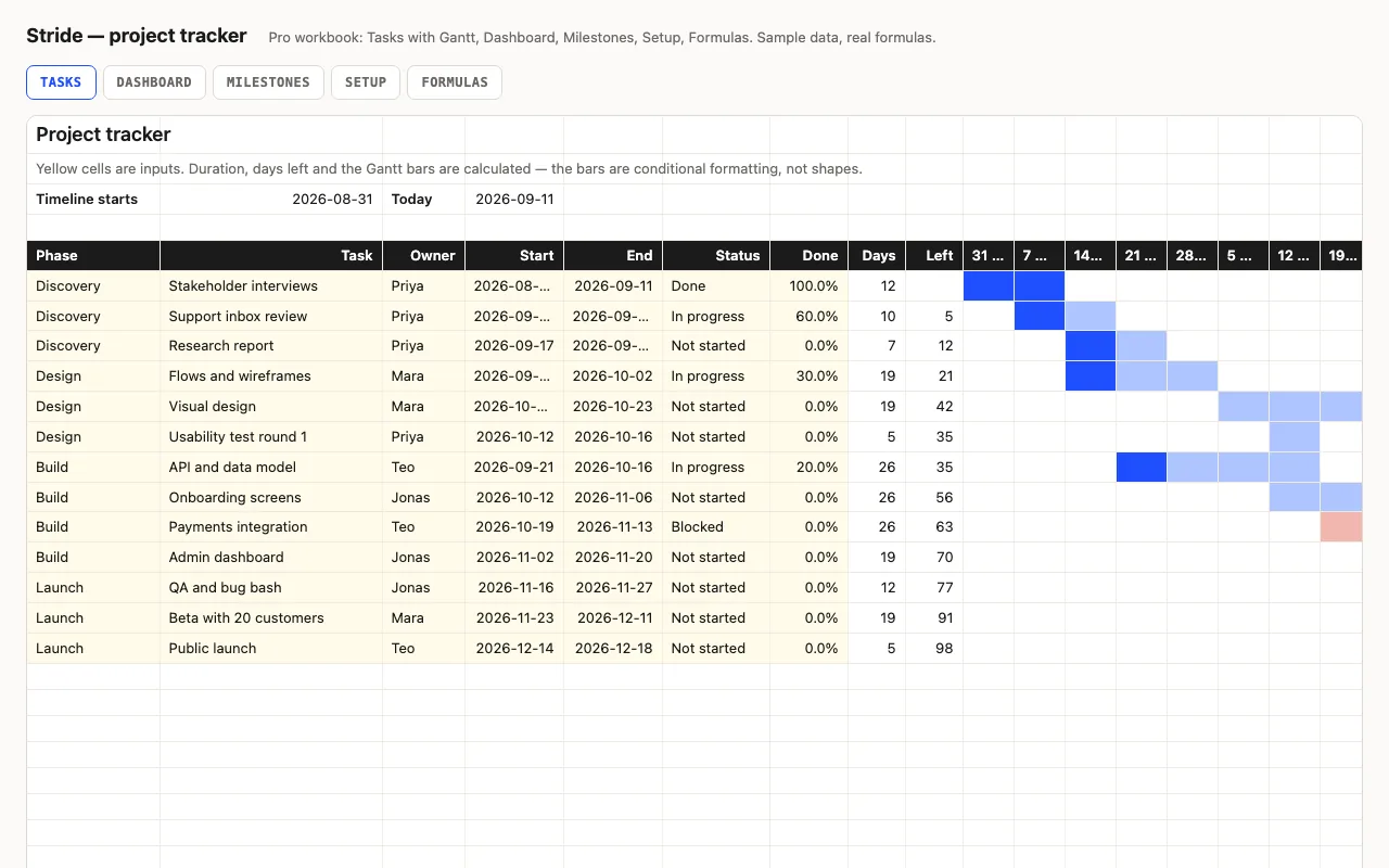
A Gantt chart is the classic macro magnet: shapes that a script positions from dates. Delete the script and the shapes freeze. The alternative is a grid of week columns, each header a Monday, and a formula that decides whether each cell is inside a task.

the planned bar: does this week overlap the task?

=AND($D6<>"",  J$5 <= $E6,  J$5+6 >= $D6)
    ↑ task has a start   ↑ week starts on/before task end   ↑ week ends on/after task start

the done part: is this week before the progress front?

=AND($D6<>"", J$5<=$E6, J$5+6>=$D6,  J$5 < $D6 + ($E6-$D6+1)*$G6)
                                     ↑ start + duration × Done%

Three rules — done, blocked, planned — in that order with “stop if true”, and a fourth that puts a red left border on the column whose week contains today. Move a date and the bar moves. Type 40% and the first 40% goes solid. Nothing to enable.

Rule 7: a filtered list without FILTER

FILTER is the tidy answer to “show only the items below their reorder point” — in Microsoft 365 and Google Sheets. Excel 2016, 2019 and Numbers don’t have it, and a template that says “Excel” should work there. The portable version mirrors the source sheet row by row:

each Reorder row mirrors the Stock row with the same number

A5:  =IF(AND(Stock!$A5<>"", Stock!$H5<=Stock!$I5), Stock!$A5, "")
B5:  =IF(AND(Stock!$A5<>"", Stock!$H5<=Stock!$I5), Stock!$B5, "")
…
Lines to order:  =COUNT(C5:C201)      ← counts the numeric on-hand cells that showed

Blank rows stay between the hits; a sort or an autofilter tightens the list if you want one. It’s less elegant than FILTER and it opens on every machine your customer has.

Rule 8: guard the divisions, round the money

=C12/$C$8 is fine until the month has no income yet, and then every percentage on the sheet is #DIV/0!. Wrap it: =IF($C$8=0, 0, C12/$C$8).

For anything that compounds — a loan schedule, running balances — round where a bank would. Interest each month is =ROUND(previous_balance * rate/12, 2), and the payment is capped at what’s owed, =MIN(scheduled, balance + interest), so the last row lands on exactly 0.00 instead of leaving three cents behind for the next 400 rows.

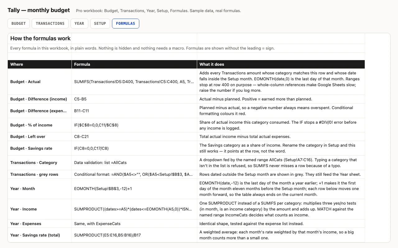
Rule 9: write the formulas down

A workbook that has to be understood by someone who didn’t build it needs one more sheet: each formula, in plain words. Which cells it reads, why the IF is there, where the range stops. It costs an hour and it is the difference between a template and a file. Write the formulas without the leading = on that sheet — otherwise Excel treats the explanation as a live formula and tries to calculate it.

Checking it

A formula you can see is a formula you can check. Three ways, cheapest first:

Change an input and watch. Add a transaction; the budget total should move by exactly that amount. Set a task to Done; its bar should go solid to the end.
Add up a column by hand for a small sample and compare with the sheet’s total.
Recalculate in a different engine. Our build opens the finished .xlsx in LibreOffice (headless) and in an independent Python formula engine, computes every cell from the sample data, compares a dozen totals against numbers a script worked out on its own, and scans every formula cell for an error value. That caught the "" bug above, a month-offset error in a twelve-month table, and a COUNTIF wildcard that behaves differently across engines — before any of them reached a buyer. LibreOffice is free; soffice --headless --convert-to xlsx is all it takes to make it recalculate a file.

Google Sheets and Numbers

Everything in this guide works in both. The functions used — SUMIFS, COUNTIFS, SUMPRODUCT, INDEX/MATCH, EOMONTH, EDATE, PMT, IFERROR — are common to Excel 2016+, Google Sheets and Numbers, as are named ranges, data validation lists, conditional formatting with formulas, and data bars. Numbers flattens named ranges to plain references on import; the formulas keep working. The two things to avoid for portability are whole-column references (Rule 4) and FILTER/XLOOKUP/LET (Rule 7).

If you’d rather start from one of ours: the five in the spreadsheets section follow every rule here, with a free sheet each and a live preview of the numbers.